The vehicle routing problem as classically formulated assumes a relatively open network where the cost of traversing an edge is a function of distance and travel time, and the primary optimization objective is minimizing total route cost across all deliveries. This formulation works reasonably well for highway-based freight and intercity distribution. It breaks down in dense urban environments in ways that are systematic, not random, and understanding why it breaks down is necessary to designing an approach that actually works in cities.
Why Urban Routing Is a Different Problem
The classical VRP formulation treats the road network as a weighted graph where the weights are stable enough to use for planning. In an urban grid, three properties of the graph undermine this assumption.
First, travel time weights are highly time-variant. A 0.8-kilometer segment through a Chicago downtown intersection might take 3 minutes at 10am and 14 minutes at 5:15pm. Using an average travel time for that segment produces routes that are correct in expectation but frequently wrong at execution. For urban delivery operations where time windows are measured in 30-minute increments, being off by 11 minutes on a single segment cascades through the entire route sequence.
Second, access constraints are location-specific and not reflected in standard road network data. Loading zone restrictions, height restrictions under rail bridges, turning radius constraints at certain intersections, commercial vehicle prohibitions on certain streets during certain hours: these are the rules that every experienced urban driver has memorized and that no commercially available routing engine has complete data on. The mismatch between the road network model and the physical reality of where commercial vehicles can legally and practically operate is larger in dense urban areas than anywhere else.
Third, service time variance is higher in urban environments. Delivering to a residential high-rise in a dense neighborhood takes longer than delivering to a suburban warehouse because parking is further from the delivery point, elevator wait times are real, and obtaining building access may require a call to a doorman or a wait at a security desk. Standard routing models use a fixed service time per stop, which is a reasonable approximation for warehouse deliveries and totally wrong for urban residential and mixed-use commercial stops.
Time-Window Compliance in Urban Operations
Time-window compliance is the metric that most directly reflects whether your routing model is accurately representing the urban environment. A fleet achieving 92% on-time delivery in suburban operations and 71% on-time in the same metropolitan area's urban core is telling you something about model quality, not just traffic variability.
The components of a time-window compliance shortfall in urban operations are usually: travel time estimation error (the model's edge weights are wrong for time of day), service time estimation error (the model underestimates how long each urban stop actually takes), and sequencing error (the model is ordering stops in a way that looks geographically efficient but creates driving path conflicts with one-way streets, restricted turns, and loading zone availability).
Separating these causes requires data that most operations do not collect systematically. Driver app data that timestamps arrival at stop, departure from stop, and any notes about access delay lets you compute actual service time versus planned service time at each location. Comparing actual versus planned travel time between consecutive stops gives you travel time estimation error. Both analyses are tractable with consistent driver app usage and produce the information you need to tune your routing model for the specific urban environment you operate in.
Turn-by-Turn Constraints and Their Routing Impact
Standard routing algorithms optimize at the street segment level: which segments to include in the route. Turn-by-turn constraints operate at the node level: which turns are allowed at each intersection. For passenger vehicles in a normal street network, this distinction rarely matters. For commercial vehicles in a dense urban area, it matters significantly.
Large trucks cannot make certain turns. Certain intersections have commercial vehicle restrictions. One-way street configurations create situations where the road network graph predicts a 200-meter path that actually requires 900 meters of routing because the direct path requires a prohibited turn or a one-way conflict. A routing model that does not account for turn-by-turn constraints generates routes that look correct on the node-to-node level and fail in navigation.
Incorporating turn restrictions into the routing graph requires a different data model. Rather than edges between nodes, you model edges between edge-pairs (what turns are allowed when arriving on one edge and departing on another). This is the standard representation for turn-restricted routing and is available in commercial mapping platforms, but it increases the graph complexity and therefore the computational cost of optimization. For urban delivery operations with many stops, the computational difference is not trivial.
The practical approach most urban delivery operations use is a hybrid: optimize at the street segment level for initial route construction, then post-process the route through a turn-compliant navigation engine to validate and correct the turn sequences. This catches the worst violations without carrying the full computational cost of turn-constrained optimization for every route generation.
Loading Zone Availability as a Routing Constraint
One of the most under-modeled constraints in urban logistics is loading zone availability. In a city like Chicago, commercial loading zones have designated hours, vehicle size limits, and time limits. A route that arrives at a delivery stop during loading zone hours has a predictable service time. The same route arriving during restricted hours requires either circling for a legal parking space or double-parking, both of which dramatically increase actual service time and create risk of a citation that is not captured in the route cost model.
Incorporating loading zone data into routing decisions is logistically complex because the data requires ongoing maintenance (loading zone rules change, zones are added or removed, temporary construction zones supersede standard zones), and the granularity required is stop-specific, not street-segment-level. It is, however, the kind of constraint that can generate outsized route quality improvement relative to the modeling effort, because loading zone violations are often the single largest source of service time variance in dense urban delivery operations.
The practical starting point is identifying which stops in your urban delivery network have the highest service time variance, and whether the variance correlates with time-of-day. A stop with high service time variance in the 8am-10am window and low variance in the 11am-2pm window is probably a loading zone availability issue. Scheduling those stops preferentially in the low-variance window is a routing adjustment that does not require a new data model, just better use of existing service time data to inform time window targeting.
What Standard Algorithms Handle Poorly and Why
This is not an argument that standard VRP algorithms are wrong for urban use cases. They are solving the problem they were designed to solve. The mismatch is between the problem formulation and the physical reality of dense urban delivery.
The formulation gap is solvable by enriching the model inputs: time-variant edge weights (learned from historical performance data), stop-specific service time estimates (derived from actual driver app data), turn restriction constraints (from commercial map data), and time-window preferences based on loading zone availability. None of this requires a new algorithm. It requires better data inputs to the existing algorithm and a routing system that can update those inputs continuously rather than running on a static snapshot of the network.
The improvement from moving to a data-enriched urban routing model is typically larger than any algorithmic upgrade alone. Most urban delivery operations are not running suboptimal algorithms; they are running good algorithms against an impoverished model of the physical environment they actually operate in.